Exaggerated Topography in Paraview
Description
The usual way of putting topography onto a model is to use a sphere (= convert lat/lon of ETOPO to cartesian coordinates) and color the grid points by their altitudes. However, the 3D shape of a mountain range can be emphasized by exaggerating the vertical dimension. This can be done of course by adding the exaggerated topography to the Earth's radius when computing cartesian coordinates.
A more elegant approach to this is: Computing the exaggerated topography on-the-fly using the Calculator filter of Paraview. This filter can do arbitrary computations with the data fields and coordinates of the models and return either a new dataset, or modify the coordinates of the grid (if the computation returns 3D vectors). The latter is exactly what we need for this task:
- Load a VTK file with the surface of the Earth, where the center is at 0/0/0 and the topography is given in a data field (here: "altitude"). Here, the radius is assumed to be normalized to 1.
- Use the "Calculator" filter, and activate the checkbox "Coordinate Results".
- Type in the appropriate formula (and replace "exaggeration" by your actual value; everything must be on one line).
- Spherical Earth (assumption: center of the Earth = 0/0/0, radius = 1):
(1 + (altitude/6370000) * exaggeration)
* ( iHat * cos(asin(coordsZ)) * cos(atan(coordsY/coordsX)) * coordsX/abs(coordsX)
+ jHat * cos(asin(coordsZ)) * sin(atan(coordsY/coordsX)) * coordsX/abs(coordsX)
+ kHat * coordsZ )
- Flat Earth: Here, things are much easier, since only the z coordinate has to be modified. Thus, the formula is:
coordsX * iHat + coordsY * jHat + altitude * kHat * exaggeration
Examples
The following example shows how to exaggerate a dataset derived from SRTM data of the region northwest of Fürth/Germany:
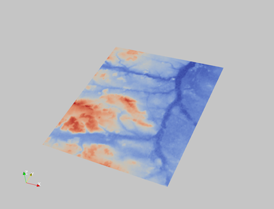
This is the SRTM dataset in a polygonal mesh, with a regular grid spacing; the mesh itself is flat, and the colors show the altitude:

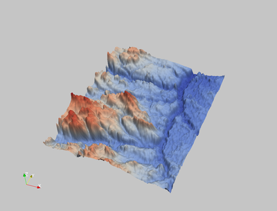
Now, let's apply the calculator filter described above, with a exaggeration factor of 25:

A normal landscape does not have sharp edges. This can be changed by computing normal vectors at the edges. These normal vectors determine the reflection of light. If there are no surface normals explicitly given, the normal vectors derived from the orientation of the facets change abruptly, so the edges are clearly visible. But there is the filter Generate Surface Normals which computes smooth transitions between adjacent facets, so the surface looks smooth even without increasing the resolution.
In the example above, Generate Surface Normals has been used with the following settings:
- Feature angle: 30°
- Consistency: yes
- Splitting: no
- Flip normals: no
- Non-manifold traversal: No
- Compute cell normals: no (not needed)
- Piece invariant: no
Now the image looks much smoother:

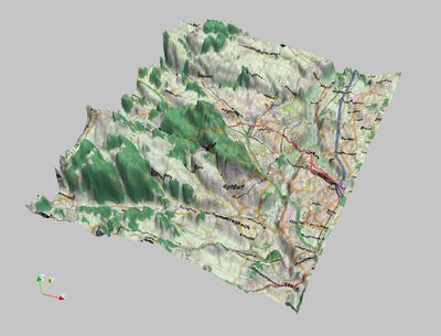
And finally we can add a map, from OpenStreetMap (see Paraview: Topography by Texture Mapping):

