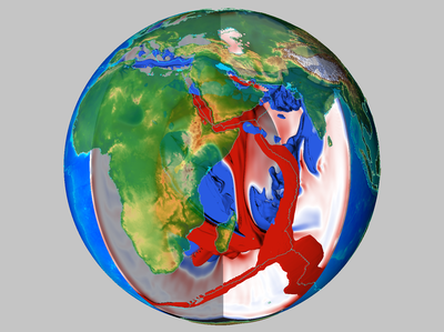
Tutorial: TERRA Model + Topography in Paraview
Step 1: Generate Paraview Files
TERRA produces output files that contain temperature, velocity and pressure. These files, albeit ASCII, have a proprietary format and do not contain any grid information. There are basically two ways to convert TERRA files into Paraview/VTK files:
- Recent TERRA versions can generate *.vtu files, one file per MPI process.
- The tool terra_export.pl, which is described in Visualization in Paraview, Gocad etc., generates Paraview files (in the old *.vtk format); it can export arbitrary layers and/or diamonds or the dataset, but not compute new surfaces.
These files can be loaded by Paraview - however, probably not on every computer, since a lot of memory is required. You have the following options:
- Use either a machine with a sufficiently high amount of RAM.
- Use a cluster (via MPI and Paraview).
- Process the pieces individually and join them only at the end when the amount of data is sufficiently reduced and the final pictures are created.
When the dataset is loaded into Paraview, it looks probably quite boring:
(This does not change even if the files are not shown with a solid color, but colored according to a data field such as temperature.)
Step 2: Remove Outer Layer
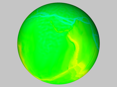
In the image above everything has the same color since the temperature is kept fixed at the boundary. So remove a tiny layer using the "Clip" filter (type: sphere; origin: 0/0/0; radius: 0.99; inside out). Now the result shows the shapes of the continents:
Step 3: Change Color Table
Temperatures are shown best with colors from blue to red. And since we have here not the absolute temperatures, but temperature deviations, it makes sense to show the average temperature. With a blue-white-red color table (white = 0), the image looks like this:
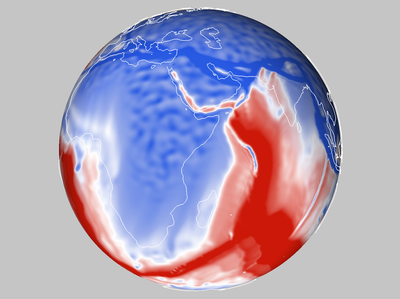
(Here, also Coastlines have been loaded.)
Step 4: Extract Cut Surfaces
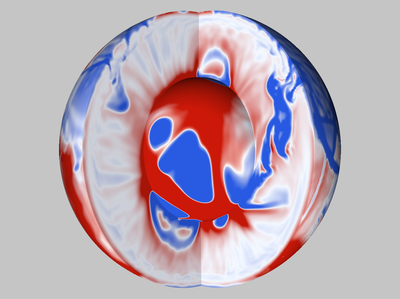
We don't need the whole amount of data; actually, just the surfaces are visible. So we can use the "Cut" and "Clip" filters:
- A spherical cut generates the core with the temperatures of the CMB.
- To cut out a part of the Earth, one can use the "Clip" filter; here, a cube with an edge along the Earth's axis is cut out. Then, the "Surface" filter has been used to extract the surface of the remaining object.
Step 5: Isosurfaces
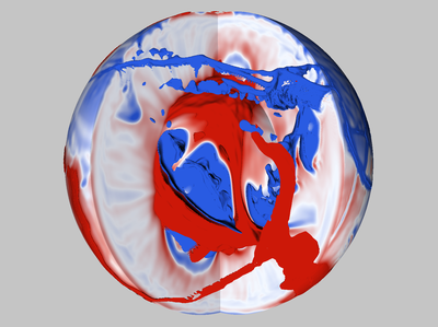
Here are two isosurfaces of the original dataset, at +400 K and -600 K, created using the "Contour" filter:
Step 6: Topography
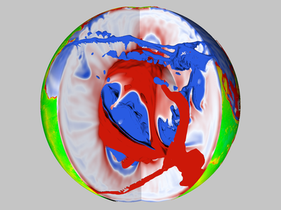
Almost every visualization of the Earth needs Topography or at least Coastlines. Here we have loaded the ETOPO dataset, and cut it in the same way as the simulation data in step 4:
Step 7: Separate Continents from Oceans
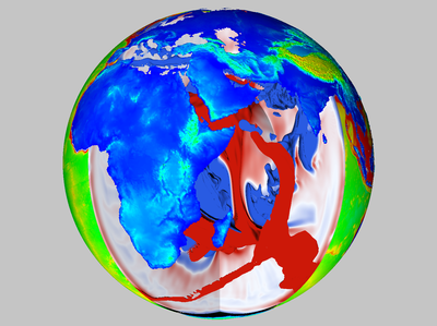
This can be done using the "Threshold" filter: Create two datasets, one with the elevations above 0 m and the other with the elevations below. And then use the clip filter from step 6 only on the oceanic part:
Step 8: Change the Colors of the Topography
Topography looks much nicer if it has the colors that we know from maps:
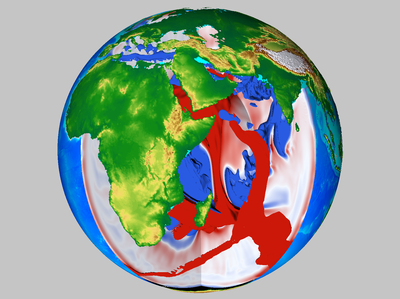
Step 9: Use Transparency
Requires a lot of fine-tuning, but can improve the result:
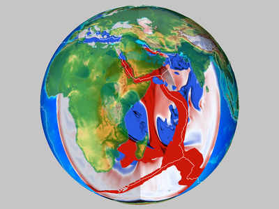
(Also plate boundaries have been added.)
Step 10: Adjust Lights
Light from the side creates shadows and increases the spatial effect:
